Matlab Demos in the Week-2 Lecture

Contents

The codes for the example in page 16 of week-1 lecture

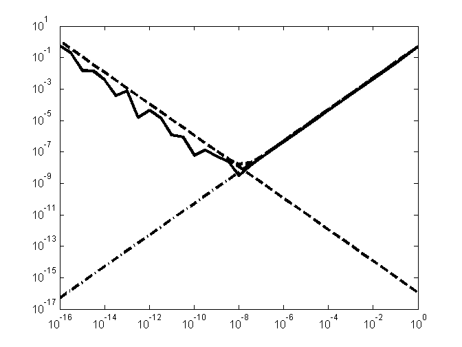
The figure demos the rounding error and truncation error in a finite-difference calculation (see page 16 of sides of lecture 1).

edit fig1_2.m
fig1_2

% codes of fig1_2.m
h=logspace(-16, 0, 33);    % sampling of h
yerr= (sin(1+h)-sin(1))./h; % finite difference
yerr= yerr-cos(1);         % error of finite difference

trunc_err= h/2;            % estimation of truncation error
round_err= eps/2*ones(size(h,1))./h; % estimation of rounding error
% plot the curves
fig=loglog(h, trunc_err, 'k-.', ...
        h, round_err, 'k--', ...
        h, abs(yerr), 'k-', ...
        h, trunc_err+round_err, 'k--');
% set linewidth, axis and ticks for better visibility
set(fig, 'linewidth', 3);
axis([1e-16, 1, 1e-17, 1e1]);
ytick=logspace(-17,1,10);
ytick(1)=1e-17;
set(gca,'xtick',logspace(-16, 0, 9), 'ytick', ytick)

Examples of floating-point numbers in computer

%0.1 can not be precisely store in computer. Here we see the hex format of its machine number.

t= 0.1;
format hex;
t

% The sum of ten 0.1 is not 1.
a=t; for i=1:9, a=a+t; end     % in hex format, 1 is 3ff0000000000000
a

format long
a

% A old formula to show the epsilon machine
x= 1-3*(4/3-1)

t =

   3fb999999999999a


a =

   3fefffffffffffff


a =

   1.000000000000000


x =

    2.220446049250313e-016

Published with MATLAB® 7.8